C3S Soil Moisture Data Access and Anomaly Analysis Notebook

In this tutorial we will download C3S Satellite Soil Moisture data from the Copernicus Climate Data Store (CDS), read data stacks in python using xarray and perform simple analyses of soil moisture anomalies over selected study areas.

The tutorial comprises the following main steps:

1. A short description of the data sets
2. Download satellite soil moisture images from CDS using the CDS API
3. Application 1: Open downloaded data and visualize the soil moisture variable
4. Application 2: Extract a time series for a single location and compute the soil moisture anomaly
5. Application 3: Vectorized anomaly computation and data extraction for a study area

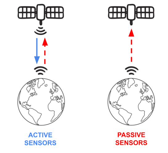
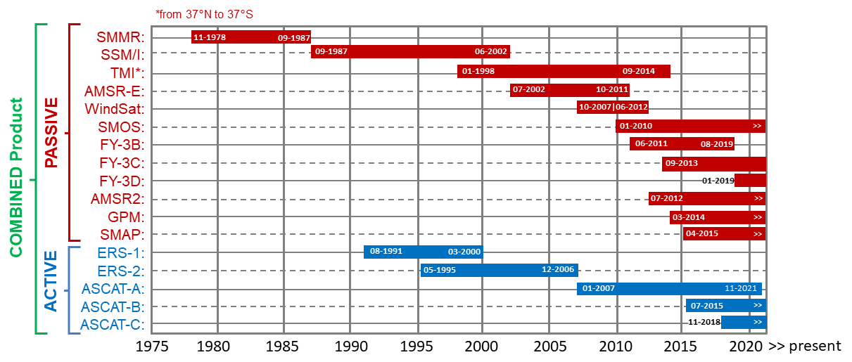
You can run this tutorial in your browser via free cloud platforms:

Note: Cells in this notebook are meant to be executed in order* (from top to bottom). Some of the later examples depend on previous ones!*

Setup

First we make sure to install the CDS API via pip by running:

%%capture --no-display
!pip install cdsapi

In the next cell we import all libraries necessary to run code in this notebook. Some of them are python standard libraries, that are installed by default. If you encounter any errors during import, you can install missing packages using the conda package manager via:

!conda install -y -c conda-forge <PACKAGE>

A full list of dependencies required to run this notebook is available in the file environment.yml at https://github.com/TUW-GEO/c3s_sm-tutorials. If you are on Binder, all necessary dependencies are already installed.

import os
import cdsapi
from pathlib import Path
import ipywidgets as widgets
import matplotlib.pyplot as plt
import cartopy
import cartopy.crs as ccrs
import xarray as xr
import shutil
import pandas as pd
import zipfile
from collections import OrderedDict

%matplotlib inline

The file utils.py is part of this package. It contains helper functions that are not relevant to understand contents of the notebook and therefore transferred to a separate file.

import utils as utils

1. About C3S Satellite Soil Moisture

Satellites sensors can observe the amount of water stored in the top layer of the soil from space. Various satellite missions from different space agencies provide measurements of radiation from the Earth's surface across different (microwave) frequency domains (e.g. Ku-, X-, C-, and L-band), which are related to the amount of water stored in the soil. There are two types of sensors that are used to measure this information: passive systems (radiometer) and active systems (radar).

For a detailed description, please see the C3S Soil Moisture Algorithm Theoretical Baseline Document, which is available together with the data at the Copernicus Climate Data Store.

Soil moisture from radiometer measurements (PASSIVE)

Brightness temperature is the observable of passive sensors (in $°K$). It is a function of kinetic temperature and emissivity. Wet soils have a higher emissivity than dry soils and therefore a higher brightness temperature. Passive soil moisture retrieval uses this difference between kinetic temperature and brightness temperature to model the amount of water available in the soil of the observed area, while taking into account factors such as the water held by vegetation.

NASA's SMAP and ESA's SMOS satellites are examples for L-band radiometer missions. They are suitable for retrieving soil moisture globally, even when vegetation is present in a scene.

Different models to retrieve Soil Moisture from brightness temperature measurements exist. One of the them is the Land Parameter Retrieval Model (Owe et al., 2008, Owe et al., 2001, and van der Schalie et al., 2016). This model is used to derive soil moisture for all passive sensors in C3S.

The PASSIVE product of C3S Soil Moisture contains merged observations from passive systems only. It is given in volumetric units $[m^3 / m^3]$.

Soil moisture from scatterometer measurements (ACTIVE)

Active systems emit radiation in the microwave domain (C-band in C3S). As the energy pulses emitted by the radar hit the Earth's surface, a scattering effect occurs and part of the energy is reflected back, containing information on the surface state of the observed scene. The received energy is called “backscatter”, with rough and wet surfaces producing stronger signals than smooth or dry surfaces. Backscatter comprises reflections from the soil surface layer (“surface scatter”), vegetation (“volume scatter”) and interactions of the two.

ESA's ERS-1 and ERS-2, as well as EUMETSAT's Metop ASCAT sensors are active systems used in C3S soil moisture. In the case of Metop ASCAT, C3S Soil Moisture uses the Surface Soil Moisture products directly provided by H SAF, based on the WARP algorithm (Wagner et al., 1999, Wagner et al., 2013).

The ACTIVE product of C3S Soil Moisture contains merged observations from active systems only. It is given in relative units $[\%$ $saturation]$.

Merged product (COMBINED)

Single-sensor products are limited by the life time of the satellite sensors. Climate change assessments, however, require the use of long-term data records, that span over multiple decades and provide consistent and comparable observations. The C3S Soil Moisture record therefore merges the observations from more than 15 sensors into one harmonized record. The main two steps of the product generation include scaling all sensors to a common reference, and subsequently merging them by applying a weighted average, where sensor with a lower error are assigned a higher weight. The following figure shows all satellite sensors merged in the PASSIVE (only radiometers), ACTIVE (only scatterometers) and COMBINED (scatterometers and radiometers) C3S product (data set version v202212).

C3S Soil Moisture is based on the ESA CCI SM algorithm, which is described in Dorigo et al., 2017 and Gruber et al., 2019.

The COMBINED product is also given in volumetric units $[m^3 / m^3]$. However, the absolute values depend on the scaling reference, which is used to bring all sensors into the same dynamic range. In this case we use Soil Moisture simulations for the first 10 cm from the GLDAS Noah model (Rodell et al., 2004).

2. Data Access and Download

Different products and versions for C3S Soil Moisture are available on the Copernicus Climate Data Store. In general, there are 2 types of data records:

• CDR: The long term Climate Data Record, processed every 1-2 years, contains data for more than 40 years, but not up-to-date.
• ICDR: Interim Climate Data Record, updated every 10-20 days, extends the CDR, contains up-to-date (harmonised) observations to append to the CDR.

Creating a valid CDS data request for satellite soil moisture

There are different options to specify a valid C3S Soil Moisture CDS data download request. You can use the CDS GUI to generate a valid request (button Show API Request) and copy/paste it into your python script as shown below. To summarize the options:

• variable: Either volumetric_surface_soil_moisture (must be chosen to download the PASSIVE or COMBINED data) or surface_soil_moisture (required for ACTIVE product)
• type_of_sensor: One of active, passive or combined_passive_and_active (must match with the selected variable!)
• time_aggregation: month_average, 10_day_average, or day_average. The original data is daily. Monthly and 10-daily averages are often required for climate analyses and therefore provided for convenience.
• year: a list of years to download data for (COMBINED and PASSIVE data is available from 1978 onward, ACTIVE starts in 1991)
• month: a list of months to download data.
• day: a list of days to download data for (note that for the monthly data, day must always be '01'. For the 10-daily average, valid days are: '01', '11', '21' (therefore the day always refers to the start of the period the data represents).
• area: (optional) Coordinates of a bounding box to download data for.
• type_of_record: cdr and/or icdr. It is recommended to select both, to use whichever data is available (there is no overlap between ICDR and CDR of a major version).
• version: Data record version, currently available: v201706.0.0, v201812.0.0, v201812.0.1, v201912.0.0, v202012.0.0, v202012.0.1, v202012.0.2 (as of January 2023, new versions are added regularly). Sub-versions indicate new data that is meant to replace the previous sub-versions (necessary e.g. due to processing errors). It is therefore recommended to pass all sub-versions and use the file with the highest version for any time stamp in case of duplicate time stamps.
• format: Either zip or tgz. Archive format that holds the individual netcdf images.

Getting your CDS API Key

In order to download data from the Climate Data Store (CDS) via the API you need:

1. An account at https://cds.climate.copernicus.eu
2. Your personal API key from https://cds.climate.copernicus.eu/api-how-to

If you do not provide a valid KEY in the next cell, the following API request will fail. However, you can then still continue with the example data provided together with this notebook, which is the same data you would get if the query is not changed: i.e., monthly volumetric surface soil moisture from passive observations at version v202012 over Europe, from CDR & ICDR. The provided example data is stored in the repository as this notebook (./DATA/sm_monthly_passive_v202012.zip). It is recommended to use monthly data, as some of the examples in this notebook will not work with daily or 10-daily images!

URL = "https://cds.climate.copernicus.eu/api/v2"
# If you have a valid key, set it in the following line:
KEY = "######################################"

In this cell we submit a data request. This will only succeed if

• a valid KEY was defined in the previous cell
• a valid request is made (the default request here is valid).

Otherwise the data request will fail. However, this is not a problem for this tutorial. We will just fall back to the data provided with this notebook.

try:
    c = cdsapi.Client(url=URL, key=KEY)
    DATA_PATH = Path("DATA") / "my_data.zip"
    c.retrieve(
        "satellite-soil-moisture",
        {
            "variable": "volumetric_surface_soil_moisture",
            "type_of_sensor": "passive",
            "time_aggregation": "month_average",  # required for examples in this notebook
            "year": [str(y) for y in range(1991, 2023)],
            "month": [f"{m:02}" for m in range(1, 13)],
            "day": "01",
            "area": [72, -11, 34, 40],
            "type_of_record": ["cdr", "icdr"],
            "version": ["v202012.0.0", "v202012.0.1", "v202012.0.2"],
            "format": "zip",
        },
        DATA_PATH,
    )
except Exception as e:
    DATA_PATH = Path("DATA") / "sm_monthly_passive_v202012.zip"
    print(
        "Could not download data from CDS using the passed request and/or API Key.\n"
        f"The following error was raised: \n   {e} \n \n"
        f"We therefore continue with the data provided in: {DATA_PATH}"
    )

2023-02-06 17:16:52,300 INFO Sending request to https://cds.climate.copernicus.eu/api/v2/resources/satellite-soil-moisture

Could not download data from CDS using the passed request and/or API Key.
The following error was raised: 
   'tuple' object is not callable 
 
We therefore continue with the data provided in: DATA/sm_monthly_passive_v202012.zip

Unpacking & Loading Data with xarray

From the previous cell, we have a variable DATA_PATH which points to a .zip archive (either newly downloaded or the one provided with this tutorial) containing the selected data from CDS as individual images. We use the library xarray to read these data, but first we have to extract them. In the next cell we extract all files from the downloaded .zip archive into a new folder. We do this using standard python libraries:

# Setting up a temporary folder to extract data to:
extracted_data = Path(f"{DATA_PATH}_extracted")
if os.path.exists(extracted_data):
    shutil.rmtree(extracted_data)
os.makedirs(extracted_data)

# Extract all files from zip:
with zipfile.ZipFile(DATA_PATH, "r") as archive:
    archive.extractall(extracted_data)

We can then use the function xarray.open_mfdataset to load all extracted files and concatenate them along the 'time' dimension automatically. This way we get a 3-dimensional (longitude, latitude, time) data cube, that we store in a global variable DS. In addition we extract the unit and valid range of the soil moisture variable from the netCDF metadata (SM_UNIT and SM_RANGE).

DS = xr.open_mfdataset(os.path.join(extracted_data, "*.nc"))
SM_UNIT = DS["sm"].attrs["units"]
SM_RANGE = DS["sm"].attrs["valid_range"]

Finally we plot a table that shows the contents of DS. You can see the dimensions of the data cube, coordinates assigned to each dimension, and data variables (each data point has coordinates assigned for each dimension). You can also explore the 'Attributes' field (i.e. metadata assigned to the data cube) by clicking on it.

DS

<xarray.Dataset>
Dimensions:     (lat: 152, lon: 204, time: 384)
Coordinates:
  * lat         (lat) float32 71.88 71.62 71.38 71.12 ... 34.62 34.38 34.12
  * lon         (lon) float32 -10.88 -10.62 -10.38 -10.12 ... 39.38 39.62 39.88
  * time        (time) datetime64[ns] 1991-01-01 1991-02-01 ... 2022-12-01
Data variables:
    sm          (time, lat, lon) float32 dask.array<chunksize=(1, 152, 204), meta=np.ndarray>
    sensor      (time, lat, lon) float32 dask.array<chunksize=(1, 152, 204), meta=np.ndarray>
    freqbandID  (time, lat, lon) float32 dask.array<chunksize=(1, 152, 204), meta=np.ndarray>
    nobs        (time, lat, lon) float32 dask.array<chunksize=(1, 152, 204), meta=np.ndarray>
Attributes: (12/40)
    title:                      C3S Surface Soil Moisture merged PASSIVE Product
    institution:                EODC (AUT); TU Wien (AUT); VanderSat B.V. (NL)
    contact:                    C3S_SM_Science@eodc.eu
    source:                     LPRMv6/SMMR/Nimbus 7 L3 Surface Soil Moisture...
    platform:                   Nimbus 7, DMSP, TRMM, AQUA, Coriolis, GCOM-W1...
    sensor:                     SMMR, SSM/I, TMI, AMSR-E, WindSat, AMSR2, SMO...
    ...                         ...
    id:                         C3S-SOILMOISTURE-L3S-SSMV-PASSIVE-MONTHLY-199...
    history:                    2021-03-29T13:46:57.630282 mean calculated
    date_created:               2021-03-29T13:46:57Z
    time_coverage_start:        1990-12-31T12:00:00Z
    time_coverage_end:          1991-01-31T12:00:00Z
    time_coverage_duration:     P1M

xarray.Dataset

• Dimensions:
  • lat: 152
  • lon: 204
  • time: 384
• Coordinates: (3)
  • lat
    (lat)
    float32
    71.88 71.62 71.38 ... 34.38 34.12

    standard_name :

    latitude

    units :

    degrees_north

    valid_range :

    [-90. 90.]

    _CoordinateAxisType :

    Lat

    array([71.875, 71.625, 71.375, 71.125, 70.875, 70.625, 70.375, 70.125, 69.875,
           69.625, 69.375, 69.125, 68.875, 68.625, 68.375, 68.125, 67.875, 67.625,
           67.375, 67.125, 66.875, 66.625, 66.375, 66.125, 65.875, 65.625, 65.375,
           65.125, 64.875, 64.625, 64.375, 64.125, 63.875, 63.625, 63.375, 63.125,
           62.875, 62.625, 62.375, 62.125, 61.875, 61.625, 61.375, 61.125, 60.875,
           60.625, 60.375, 60.125, 59.875, 59.625, 59.375, 59.125, 58.875, 58.625,
           58.375, 58.125, 57.875, 57.625, 57.375, 57.125, 56.875, 56.625, 56.375,
           56.125, 55.875, 55.625, 55.375, 55.125, 54.875, 54.625, 54.375, 54.125,
           53.875, 53.625, 53.375, 53.125, 52.875, 52.625, 52.375, 52.125, 51.875,
           51.625, 51.375, 51.125, 50.875, 50.625, 50.375, 50.125, 49.875, 49.625,
           49.375, 49.125, 48.875, 48.625, 48.375, 48.125, 47.875, 47.625, 47.375,
           47.125, 46.875, 46.625, 46.375, 46.125, 45.875, 45.625, 45.375, 45.125,
           44.875, 44.625, 44.375, 44.125, 43.875, 43.625, 43.375, 43.125, 42.875,
           42.625, 42.375, 42.125, 41.875, 41.625, 41.375, 41.125, 40.875, 40.625,
           40.375, 40.125, 39.875, 39.625, 39.375, 39.125, 38.875, 38.625, 38.375,
           38.125, 37.875, 37.625, 37.375, 37.125, 36.875, 36.625, 36.375, 36.125,
           35.875, 35.625, 35.375, 35.125, 34.875, 34.625, 34.375, 34.125],
          dtype=float32)

  • lon
    (lon)
    float32
    -10.88 -10.62 ... 39.62 39.88

    standard_name :

    longitude

    units :

    degrees_east

    valid_range :

    [-180. 180.]

    _CoordinateAxisType :

    Lon

    array([-10.875, -10.625, -10.375, ...,  39.375,  39.625,  39.875],
          dtype=float32)

  • time
    (time)
    datetime64[ns]
    1991-01-01 ... 2022-12-01

    standard_name :

    time

    _CoordinateAxisType :

    Time

    array(['1991-01-01T00:00:00.000000000', '1991-02-01T00:00:00.000000000',
           '1991-03-01T00:00:00.000000000', ..., '2022-10-01T00:00:00.000000000',
           '2022-11-01T00:00:00.000000000', '2022-12-01T00:00:00.000000000'],
          dtype='datetime64[ns]')

• Data variables: (4)
  • sm
    (time, lat, lon)
    float32
    dask.array<chunksize=(1, 152, 204), meta=np.ndarray>

    dtype :

    float32

    units :

    m3 m-3

    valid_range :

    [0. 1.]

    long_name :

    Volumetric Soil Moisture

    _CoordinateAxes :

    time lat lon

    Array Chunk Bytes 45.42 MiB 121.12 kiB Shape (384, 152, 204) (1, 152, 204) Dask graph 384 chunks in 769 graph layers Data type float32 numpy.ndarray

  • sensor
    (time, lat, lon)
    float32
    dask.array<chunksize=(1, 152, 204), meta=np.ndarray>

    dtype :

    int16

    long_name :

    Sensor

    _CoordinateAxes :

    time lat lon

    flag_values :

    [0 2]

    flag_meanings :

    ['NaN', 'SSMI']

    valid_range :

    [ 0 16383]

    Array Chunk Bytes 45.42 MiB 121.12 kiB Shape (384, 152, 204) (1, 152, 204) Dask graph 384 chunks in 769 graph layers Data type float32 numpy.ndarray

  • freqbandID
    (time, lat, lon)
    float32
    dask.array<chunksize=(1, 152, 204), meta=np.ndarray>

    dtype :

    int16

    long_name :

    Frequency Band Identification

    _CoordinateAxes :

    time lat lon

    flag_values :

    [ 0 128]

    flag_meanings :

    ['NaN', 'K194']

    valid_range :

    [ 0 511]

    Array Chunk Bytes 45.42 MiB 121.12 kiB Shape (384, 152, 204) (1, 152, 204) Dask graph 384 chunks in 769 graph layers Data type float32 numpy.ndarray

  • nobs
    (time, lat, lon)
    float32
    dask.array<chunksize=(1, 152, 204), meta=np.ndarray>

    long_name :

    Number of valid observation

    CoordinateAxes :

    time lat lon

    Array Chunk Bytes 45.42 MiB 121.12 kiB Shape (384, 152, 204) (1, 152, 204) Dask graph 384 chunks in 769 graph layers Data type float32 numpy.ndarray

• Indexes: (3)
  • lat
    PandasIndex

    PandasIndex(Float64Index([71.875, 71.625, 71.375, 71.125, 70.875, 70.625, 70.375, 70.125,
                  69.875, 69.625,
                  ...
                  36.375, 36.125, 35.875, 35.625, 35.375, 35.125, 34.875, 34.625,
                  34.375, 34.125],
                 dtype='float64', name='lat', length=152))

  • lon
    PandasIndex

    PandasIndex(Float64Index([-10.875, -10.625, -10.375, -10.125,  -9.875,  -9.625,  -9.375,
                   -9.125,  -8.875,  -8.625,
                  ...
                   37.625,  37.875,  38.125,  38.375,  38.625,  38.875,  39.125,
                   39.375,  39.625,  39.875],
                 dtype='float64', name='lon', length=204))

  • time
    PandasIndex

    PandasIndex(DatetimeIndex(['1991-01-01', '1991-02-01', '1991-03-01', '1991-04-01',
                   '1991-05-01', '1991-06-01', '1991-07-01', '1991-08-01',
                   '1991-09-01', '1991-10-01',
                   ...
                   '2022-03-01', '2022-04-01', '2022-05-01', '2022-06-01',
                   '2022-07-01', '2022-08-01', '2022-09-01', '2022-10-01',
                   '2022-11-01', '2022-12-01'],
                  dtype='datetime64[ns]', name='time', length=384, freq=None))

• Attributes: (40)

  title :

  C3S Surface Soil Moisture merged PASSIVE Product

  institution :

  EODC (AUT); TU Wien (AUT); VanderSat B.V. (NL)

  contact :

  C3S_SM_Science@eodc.eu

  source :

  LPRMv6/SMMR/Nimbus 7 L3 Surface Soil Moisture, Ancillary Params, and quality flags; LPRMv6/SSMI/F08, F11, F13 DMSP L3 Surface Soil Moisture, Ancillary Params, and quality flags; LPRMv6/TMI/TRMM L2 Surface Soil Moisture, Ancillary Params, and QC; LPRMv6/AMSR-E/Aqua L2B Surface Soil Moisture, Ancillary Params, and QC; LPRMv6/WINDSAT/CORIOLIS L2 Surface Soil Moisture, Ancillary Params, and QC; LPRMv6/AMSR2/GCOM-W1 L3 Surface Soil Moisture, Ancillary Params; LPRMv6/SMOS/MIRAS L3 Surface Soil Moisture, CATDS Level 3 Brightness Temperatures (L3TB) version 300 RE03 & RE04; LPRMv6/SMAP_radiometer/SMAP L2 Surface Soil Moisture, Ancillary Params, and QC;

  platform :

  Nimbus 7, DMSP, TRMM, AQUA, Coriolis, GCOM-W1, MIRAS, SMAP

  sensor :

  SMMR, SSM/I, TMI, AMSR-E, WindSat, AMSR2, SMOS, SMAP_radiometer

  references :

  https://climate.copernicus.eu/; Dorigo, W.A., Wagner, W., Albergel, C., Albrecht, F., Balsamo, G., Brocca, L., Chung, D., Ertl, M., Forkel, M., Gruber, A., Haas, E., Hamer, D. P. Hirschi, M., Ikonen, J., De Jeu, R. Kidd, R. Lahoz, W., Liu, Y.Y., Miralles, D., Lecomte, P. (2017) ESA CCI Soil Moisture for improved Earth system understanding: State-of-the art and future directions. In Remote Sensing of Environment, 2017, ISSN 0034-4257, https://doi.org/10.1016/j.rse.2017.07.001; Gruber, A., Scanlon, T., van der Schalie, R., Wagner, W., Dorigo, W. (2019) Evolution of the ESA CCI Soil Moisture Climate Data Records and their underlying merging methodology. Earth System Science Data 11, 717-739, https://doi.org/10.5194/essd-11-717-2019; Gruber, A., Dorigo, W. A., Crow, W., Wagner W. (2017). Triple Collocation-Based Merging of Satellite Soil Moisture Retrievals. IEEE Transactions on Geoscience and Remote Sensing. PP. 1-13. https://doi.org/10.1109/TGRS.2017.2734070

  product_version :

  v202012

  tracking_id :

  544b60cc-22aa-4d83-bef2-32e653cdd226

  Conventions :

  CF-1.7

  standard_name_vocabulary :

  NetCDF Climate and Forecast (CF) Metadata Convention

  summary :

  The data set was produced with funding from the Copernicus Climate Change Service.

  keywords :

  Soil Moisture/Water Content

  naming_authority :

  EODC GmbH

  keywords_vocabulary :

  NASA Global Change Master Directory (GCMD) Science Keywords

  cdm_data_type :

  Grid

  comment :

  These data were produced as part of the Copernicus Climate Change Service. Service Contract No 2018/C3S_312b_LOT4_EODC/SC2

  creator_name :

  Earth Observation Data Center (EODC)

  creator_url :

  https://www.eodc.eu

  creator_email :

  C3S_SM_Science@eodc.eu

  project :

  Copernicus Climate Change Service.

  license :

  Copernicus Data License

  time_coverage_resolution :

  P1D

  geospatial_lat_min :

  -90.0

  geospatial_lat_max :

  90.0

  geospatial_lon_min :

  -180.0

  geospatial_lon_max :

  180.0

  geospatial_vertical_min :

  0.0

  geospatial_vertical_max :

  0.0

  geospatial_lat_units :

  degrees_north

  geospatial_lon_units :

  degrees_east

  geospatial_lat_resolution :

  0.25 degree

  geospatial_lon_resolution :

  0.25 degree

  spatial_resolution :

  25km

  id :

  C3S-SOILMOISTURE-L3S-SSMV-PASSIVE-MONTHLY-19910101000000-TCDR-v202012.0.0.nc

  history :

  2021-03-29T13:46:57.630282 mean calculated

  date_created :

  2021-03-29T13:46:57Z

  time_coverage_start :

  1990-12-31T12:00:00Z

  time_coverage_end :

  1991-01-31T12:00:00Z

  time_coverage_duration :

  P1M

Application 1: Data Visualization

Now that we have a data cube to work with, we can start by visualizing some of the soil moisture data. In this first example we create an interactive map, to show the absolute soil moisture values for a certain date. In addition we will use this example to define some locations and study areas we can use in the rest of the notebook and display their location on the map.

Study areas

First we define some potential study areas that we can use in the following examples. Below you can find a list of bounding boxes, plus one 'focus point' in each bounding box. You can add your own study area to the end of the list. If you do, make sure to pass the coordinates in the correct order: Each line consists of:

• A name for the study area
• WGS84 coordinates of corner points of a bounding box around the study area
• WGS84 coordinates of a single point in the study area

(<STUDY_AREA_NAME>, ([<BBOX min. Lon.>, <BBOX max. Lon.>, <BBOX min. Lat.>, <BBOX max. Lat.>], [<POINT Lon.>, <POINT Lat.>]))

BBOXES = OrderedDict(
    [
        # (Name, ([min Lon., max Lon., min Lat., max Lat.], [Lon, Lat])),
        ("Balkans", ([16, 29, 36, 45], [24, 42])),
        ("Cental Europe", ([6, 22.5, 46, 51], [15, 49.5])),
        ("France", ([-4.8, 8.4, 42.3, 51], [4, 47])),
        ("Germany", ([6, 15, 47, 55], [9, 50])),
        ("Iberian Peninsula", ([-10, 3.4, 36, 44.4], [-5.4, 41.3])),
        ("Italy", ([7, 19.0, 36.7, 47.0], [12.8, 43.4])),
        ("S-UK & N-France", ([-5.65, 2.5, 48, 54], [0, 51])),
    ]
)

Using ipython widgets, we can add interactive controls to our map. For the first application, we create a slider that changes the date to plot. We also include a drop down selection for one of the previously defined study areas.

dates = [str(pd.to_datetime(t).date()) for t in DS["time"].values]
SLIDER = widgets.SelectionSlider(
    options=dates,
    value=dates[-1],
    description="Select a date to plot:",
    continuous_update=False,
    style={"description_width": "initial"},
    layout=widgets.Layout(width="40%"),
)

AREA = widgets.Dropdown(options=list(BBOXES.keys()), value="Germany", description="Study Area:")

Our data cube DS is an xarray.Dataset, which comes with a lot of functionalities. For example we can create a simple map visualization of soil moisture and the number of observations for a certain date (note that nobs is only available for monthly and 10-daily averaged data downloaded from CDS). Here we extract an image from the data cube using the xarray.Dataset.sel method.

Note that the study area that is finally chosen in this example is stored in the global variable STUDY_AREA, which is again used later on in the notebook!

STUDY_AREA = None


@widgets.interact(date=SLIDER, area=AREA)
def plot_soil_moisture(date: str, area: str):
    """
    Plot the `soil moisture` and `nobs` variable of the previously loaded Dataset.
    """
    fig, axs = plt.subplots(1, 2, figsize=(17, 5), subplot_kw={"projection": ccrs.PlateCarree()})

    # Extract and plot soil moisture image for chosen date using Dataset.sel and Dataset.plot:
    p_sm = (
        DS["sm"]
        .sel(time=date)
        .plot(
            transform=ccrs.PlateCarree(),
            ax=axs[0],
            cmap=utils.CM_SM,
            cbar_kwargs={"label": f"Soil Moisture [{SM_UNIT}]"},
        )
    )
    axs[0].set_title(f"{date} - Soil Moisture")

    # Extract and plot 'nobs' image for chosen date:
    if "nobs" in DS.variables:
        # Note: nobs is only available for monthly and 10-daily data
        p_obs = (
            DS["nobs"]
            .sel(time=date)
            .plot(
                transform=ccrs.PlateCarree(),
                ax=axs[1],
                vmax=31,
                vmin=0,
                cmap=plt.get_cmap("YlGnBu"),
                cbar_kwargs={"label": "Days with valid observations"},
            )
        )
        axs[1].set_title(f"{date} - Data coverage")
    else:
        p_obs = None

    bbox = BBOXES[area][0]
    point = BBOXES[area][1]

    # Add basemape features:
    for p in [p_sm, p_obs]:
        if p is None:
            continue
        p.axes.add_feature(cartopy.feature.LAND, zorder=0, facecolor="gray")
        p.axes.coastlines()

    # Add focus point of study area to first map:
    axs[0].plot(
        [point[0]],
        [point[1]],
        color="red",
        marker="X",
        markersize=10,
        transform=ccrs.PlateCarree(),
    )
    # Add study area bounding box to first map:
    axs[0].plot(
        [bbox[0], bbox[0], bbox[1], bbox[1], bbox[0]],
        [bbox[2], bbox[3], bbox[3], bbox[2], bbox[2]],
        color="red",
        linewidth=3,
        transform=ccrs.PlateCarree(),
    )

    # Draw grid lines and labels for both maps:
    for ax in axs:
        if ax is not None:
            gl = ax.gridlines(crs=ccrs.PlateCarree(), draw_labels=True, alpha=0.25)
            gl.top_labels, gl.right_labels = False, False

    # Set global variable (to access in later examples)
    global STUDY_AREA
    STUDY_AREA = {"name": area, "bbox": bbox, "point": point}

When browsing through the images of different dates, you can see data gaps (gray areas; especially in winter, mountainous regions and high latitude) and areas of high (blue) and low (brown) soil moisture content (left map). It can be seen that the number of observations is much larger in later periods of the record than in earlier ones due to the larger number of available satellites (right map).

Application 2: Time Series Extraction and Analysis

In the following two examples we use the study area selected in Example 1. We use the chosen 'focus point' assigned to the study area (marked by the red X in the left map of the previous example) to extract a time series from the loaded stack at this location. We then compute the climatological mean (and standard deviation) for the chosen time series using the selected reference period. Finally, we subtract the climatology from the absolute soil moisture to derive a time series of anomalies. Anomalies therefore indicate the deviation of a single observation from the average (normal) conditions. A positive anomaly can be interpreted as "wetter than usual" soil moisture conditions, while a negative anomaly indicates "drier than usual" states.

There are different ways to express anomalies. For example:

1. Absolute Anomalies: Derived using the difference between the absolute values for a month ($i$) and year ($k$) ($SM_{k,i}$) and the climatology for the same month ($SM_i$). Same unit as the input data.

   $\Large SMA_{k,i}^{abs} = SM_{k,i} - \overline{SM_i}$
   

2. Relative Anomalies: The anomalies are expressed relative to the climatological mean for a month ($SM_i$), i.e. in % above / below the expected conditions.

   $\Large SMA_{k,i}^{rel}=\frac{SM_{k,i} - \overline{SM_i}}{\overline{SM_i}} \cdot 100\% $
   

3. Z-Scores: Z-scores are a way of standardizing values from different normal distributions. In the case of soil moisture, the spread of values between months can vary, e.g. due to differences in data coverage (i.e. a different distribution for values in summer than for those in winter is expected). This can affect the computed climatology and therefore the derived anomalies. By taking into account the standard deviation ($\sigma$) of samples used to compute the climatologies, we can normalize the anomalies and exclude this effect. Z-scores therefore express the number of standard deviations a value is above / below the expected value for a month.

   $\Large Z_{k,i} = \frac{SM_{k,i} - \overline{SM_i}}{\sigma_{i}}$
   

Also for this example we add interactive controls to the following plots:

• A slider to choose the baseline period
• A drop down field to select one of the above described anomaly metrics.

baseline_sider = widgets.IntRangeSlider(
    min=1991,
    max=2021,
    value=[1991, 2020],
    step=1,
    style={"description_width": "initial"},
    continuous_update=False,
    description="Climatology reference / baseline period [year from, year to]:",
    layout=widgets.Layout(width="60%"),
)

metric_dropdown = widgets.Dropdown(
    options=["Absolute Anomalies", "Relative Anomalies", "Z-Scores"],
    value="Absolute Anomalies",
    description="Metric:",
)

The next cell contains the application with the assigned widget controls.

In the first part, we extract a time series for the chosen focus point of the study area (see location in previous example).

We then select data for the chosen baseline period from the extracted time series to compute the climatology.

Using the formulas from above, we compute the three anomaly metrics for the extracted time series and store them in a pandas DataFrame (columns 'abs_anomaly', 'rel_anomaly' and 'z-score').

In the last part of the application we create the plots:

• One to show the extracted soil moisture time series (top)
• One for the climatology - the mean and standard deviation for each month in the chosen baseline period (middle)
• One for the chosen metric derived from the extracted time series and climatology (bottom)

@widgets.interact(baseline=baseline_sider, metric=metric_dropdown)
def plot_ts_components(baseline: tuple, metric: str):
    """
    Compute and visualise climatology and anomalies for the loaded soil moisture
    time series at the study area focus point.
    """
    # Extract data at location of study area 'focus point':
    lon, lat = float(STUDY_AREA["point"][0]), float(STUDY_AREA["point"][1])
    ts = DS["sm"].sel(lon=lon, lat=lat, method="nearest").to_pandas()

    # Compute scores all scores (climatology, abs. / rel. anomalies, z-scores):
    clim_data = ts.loc[f"{baseline[0]}-01-01":f"{baseline[1]}-12-31"]
    clim_std = pd.Series(clim_data.groupby(clim_data.index.month).std(), name="climatology_std")
    clim_mean = pd.Series(clim_data.groupby(clim_data.index.month).mean(), name="climatology")

    ts = pd.DataFrame(ts, columns=["sm"]).join(on=ts.index.month, other=clim_mean)
    ts["climatology_std"] = ts.join(on=ts.index.month, other=clim_std)["climatology_std"]
    ts["abs_anomaly"] = ts["sm"] - ts["climatology"]
    ts["rel_anomaly"] = (ts["sm"] - ts["climatology"]) / ts["climatology"] * 100
    ts["z_score"] = (ts["sm"] - ts["climatology"]) / ts["climatology_std"]

    # Generate three time series plots (absolute SM, climatology, chosen metric):
    fig, axs = plt.subplots(3, 1, figsize=(10, 7))

    ts["sm"].plot(
        ax=axs[0],
        title=f"Soil Moisture at focus point of `{STUDY_AREA['name']}` study area "
        f"(Lon: {lon}° W, Lat: {lat}° N)",
        ylabel=f"SM $[{SM_UNIT}]$",
        xlabel="Time [year]",
    )

    for i, g in clim_data.groupby(clim_data.index.year):
        axs[1].plot(range(1, 13), g.values, alpha=0.2)

    clim_mean.plot(
        ax=axs[1],
        color="blue",
        title=f"Soil Moisture Climatology at Lon: {lon}° W, Lat: {lat}° N",
        ylabel=f"SM $[{SM_UNIT}]$",
        label="mean",
    )
    clim_std.plot(ax=axs[1], label="std.dev. $\sigma$", xlabel="Time [month]")
    axs[1].legend()

    if metric == "Absolute Anomalies":
        var, ylabel = "abs_anomaly", f"Anomaly $[{SM_UNIT}]$"
    elif metric == "Relative Anomalies":
        var, ylabel = "rel_anomaly", "Anomaly $[\%]$"
    elif metric == "Z-Scores":
        var, ylabel = "z_score", "Z-score $[\sigma]$"
    else:
        raise NotImplementedError(f"{metric} is not implemented")

    axs[2].axhline(0, color="k")
    axs[2].fill_between(ts[var].index, ts[var].values, where=ts[var].values >= 0, color="blue")
    axs[2].fill_between(ts[var].index, ts[var].values, where=ts[var].values < 0, color="red")
    axs[2].set_ylabel(ylabel)
    axs[2].set_xlabel("Time [year]")
    axs[2].set_title(f"Soil Moisture {metric} at Lon: {lon}° W, Lat: {lat}° N")

    plt.tight_layout()

You can try and choose a different study area in the first example before re-running the above code. This will change the input data and plot anomalies for a different 'focus point'. You can also change the baseline period and see how it affects the climatology (and anomaly) computation. Choosing different anomaly metrics will change the unit of the last plot (y-axis) and lead to some differences in the time series.

Application 3: Vectorized Anomaly Computation

We now compute the the anomalies for the whole image stack (not only on a time series basis as in the previous example). For this we use some of the functions provided by xarray to group data. For the climatology (reference) we use all data from 1991 to 2020 (standard baseline period), but you can of course try a different period here as well by changing the years in the next cell. We then select all (absolute) soil moisture values in this period and group them by their month (i.e. all January, February, ... values for all years in the baseline period) and compute the mean for each group. This way we get a stack of 12 images (one for each month).

baseline = (1991, 2020)
baseline_slice = slice(f"{baseline[0]}-01-01", f"{baseline[1]}-12-31")
CLIM = DS.sel(time=baseline_slice)["sm"].groupby(DS.sel(time=baseline_slice).time.dt.month).mean()

CLIM

<xarray.DataArray 'sm' (month: 12, lat: 152, lon: 204)>
dask.array<stack, shape=(12, 152, 204), dtype=float32, chunksize=(1, 152, 204), chunktype=numpy.ndarray>
Coordinates:
  * lat      (lat) float32 71.88 71.62 71.38 71.12 ... 34.88 34.62 34.38 34.12
  * lon      (lon) float32 -10.88 -10.62 -10.38 -10.12 ... 39.38 39.62 39.88
  * month    (month) int64 1 2 3 4 5 6 7 8 9 10 11 12
Attributes:
    dtype:            float32
    units:            m3 m-3
    valid_range:      [0. 1.]
    long_name:        Volumetric Soil Moisture
    _CoordinateAxes:  time lat lon

xarray.DataArray

'sm'

• month: 12
• lat: 152
• lon: 204

• dask.array<chunksize=(1, 152, 204), meta=np.ndarray>

  Array Chunk Bytes 1.42 MiB 121.12 kiB Shape (12, 152, 204) (1, 152, 204) Dask graph 12 chunks in 831 graph layers Data type float32 numpy.ndarray

• Coordinates: (3)
  • lat
    (lat)
    float32
    71.88 71.62 71.38 ... 34.38 34.12

    standard_name :

    latitude

    units :

    degrees_north

    valid_range :

    [-90. 90.]

    _CoordinateAxisType :

    Lat

    array([71.875, 71.625, 71.375, 71.125, 70.875, 70.625, 70.375, 70.125, 69.875,
           69.625, 69.375, 69.125, 68.875, 68.625, 68.375, 68.125, 67.875, 67.625,
           67.375, 67.125, 66.875, 66.625, 66.375, 66.125, 65.875, 65.625, 65.375,
           65.125, 64.875, 64.625, 64.375, 64.125, 63.875, 63.625, 63.375, 63.125,
           62.875, 62.625, 62.375, 62.125, 61.875, 61.625, 61.375, 61.125, 60.875,
           60.625, 60.375, 60.125, 59.875, 59.625, 59.375, 59.125, 58.875, 58.625,
           58.375, 58.125, 57.875, 57.625, 57.375, 57.125, 56.875, 56.625, 56.375,
           56.125, 55.875, 55.625, 55.375, 55.125, 54.875, 54.625, 54.375, 54.125,
           53.875, 53.625, 53.375, 53.125, 52.875, 52.625, 52.375, 52.125, 51.875,
           51.625, 51.375, 51.125, 50.875, 50.625, 50.375, 50.125, 49.875, 49.625,
           49.375, 49.125, 48.875, 48.625, 48.375, 48.125, 47.875, 47.625, 47.375,
           47.125, 46.875, 46.625, 46.375, 46.125, 45.875, 45.625, 45.375, 45.125,
           44.875, 44.625, 44.375, 44.125, 43.875, 43.625, 43.375, 43.125, 42.875,
           42.625, 42.375, 42.125, 41.875, 41.625, 41.375, 41.125, 40.875, 40.625,
           40.375, 40.125, 39.875, 39.625, 39.375, 39.125, 38.875, 38.625, 38.375,
           38.125, 37.875, 37.625, 37.375, 37.125, 36.875, 36.625, 36.375, 36.125,
           35.875, 35.625, 35.375, 35.125, 34.875, 34.625, 34.375, 34.125],
          dtype=float32)

  • lon
    (lon)
    float32
    -10.88 -10.62 ... 39.62 39.88

    standard_name :

    longitude

    units :

    degrees_east

    valid_range :

    [-180. 180.]

    _CoordinateAxisType :

    Lon

    array([-10.875, -10.625, -10.375, ...,  39.375,  39.625,  39.875],
          dtype=float32)

  • month
    (month)
    int64
    1 2 3 4 5 6 7 8 9 10 11 12

    array([ 1,  2,  3,  4,  5,  6,  7,  8,  9, 10, 11, 12])

• Indexes: (3)
  • lat
    PandasIndex

    PandasIndex(Float64Index([71.875, 71.625, 71.375, 71.125, 70.875, 70.625, 70.375, 70.125,
                  69.875, 69.625,
                  ...
                  36.375, 36.125, 35.875, 35.625, 35.375, 35.125, 34.875, 34.625,
                  34.375, 34.125],
                 dtype='float64', name='lat', length=152))

  • lon
    PandasIndex

    PandasIndex(Float64Index([-10.875, -10.625, -10.375, -10.125,  -9.875,  -9.625,  -9.375,
                   -9.125,  -8.875,  -8.625,
                  ...
                   37.625,  37.875,  38.125,  38.375,  38.625,  38.875,  39.125,
                   39.375,  39.625,  39.875],
                 dtype='float64', name='lon', length=204))

  • month
    PandasIndex

    PandasIndex(Int64Index([1, 2, 3, 4, 5, 6, 7, 8, 9, 10, 11, 12], dtype='int64', name='month'))

• Attributes: (5)

  dtype :

  float32

  units :

  m3 m-3

  valid_range :

  [0. 1.]

  long_name :

  Volumetric Soil Moisture

  _CoordinateAxes :

  time lat lon

We can now use the climatology stack and compute the difference between each image of absolute soil moisture and the climatological mean of the same month. We assign the result to a new variable in the same stack called sm_anomaly. This way we compute the anomalies for the whole data cube, without a time-consuming loop over all individual locations.

%%capture --no-display
DS["sm_anomaly"] = DS["sm"] - CLIM.sel(month=DS.time.dt.month).drop("month")

We can use the bounding box chosen in the previous example to extract all soil moisture data in this area. We then compute the mean over all locations in the bounding box to get a single time series for the study area. Note that the coverage of C3S Soil Moisture varies over time (see the previous examples), which can also affect the value range of computed anomalies (standard deviation $\sigma$ is is usually larger for earlier periods).

subset = DS[["sm_anomaly"]].sel(
    lon=slice(STUDY_AREA["bbox"][0], STUDY_AREA["bbox"][1]),
    lat=slice(STUDY_AREA["bbox"][3], STUDY_AREA["bbox"][2]),
)
MEAN_TS = subset.mean(dim=["lat", "lon"]).to_pandas()
STD_TS = subset.std(dim=["lat", "lon"]).to_pandas()

Also in this example we use interactive controls to browse through individual months to visualize (same as in Application 1).

dates = [str(pd.to_datetime(t).date()) for t in DS["time"].values]
SLIDER = widgets.SelectionSlider(
    options=dates,
    value=dates[-1],
    description="Select a date to plot (map):",
    continuous_update=False,
    style={"description_width": "initial"},
    layout=widgets.Layout(width="40%"),
)

Now we can not only visualize the monthly anomalies from the processed anomaly stack, but also create a plot of annual mean values using the created time series for the whole study area bounding box.

@widgets.interact(date=SLIDER)
def plot_anomaly(date: str):
    STUDY_AREA_TS = pd.DataFrame(MEAN_TS["sm_anomaly"]).resample("A").mean()
    STUDY_AREA_TS.index = STUDY_AREA_TS.index.year

    fig = plt.figure(figsize=(15, 4), constrained_layout=True)
    gs = fig.add_gridspec(1, 3)
    map_ax = fig.add_subplot(gs[0, 0], projection=ccrs.PlateCarree())
    ts_ax = fig.add_subplot(gs[0, 1:])

    # Plot overview map by extracting data from anomaly stack for the chosen date:
    DS["sm_anomaly"].sel(time=date).plot(
        transform=ccrs.PlateCarree(),
        ax=map_ax,
        cmap=plt.get_cmap("RdBu"),
        cbar_kwargs={"label": f"Anomaly [{SM_UNIT}]"},
    )
    map_ax.axes.add_feature(cartopy.feature.LAND, zorder=0, facecolor="gray")
    map_ax.axes.coastlines()
    map_ax.add_feature(cartopy.feature.BORDERS)
    map_ax.set_title(f"{date} - Soil Moisture Anomaly")

    # Add study area box to map & add grid to map:
    bbox = STUDY_AREA["bbox"]
    map_ax.plot(
        [bbox[0], bbox[0], bbox[1], bbox[1], bbox[0]],
        [bbox[2], bbox[3], bbox[3], bbox[2], bbox[2]],
        color="red",
        linewidth=3,
        transform=ccrs.PlateCarree(),
    )
    gl = map_ax.gridlines(crs=ccrs.PlateCarree(), draw_labels=True, alpha=0.25)
    gl.right_labels, gl.top_labels = False, False

    # Create the bar plot on the right from the processed study area time series:
    bars = STUDY_AREA_TS.plot(
        kind="bar",
        ax=ts_ax,
        title=f"Annual conditions in `{STUDY_AREA['name']}` study area",
        legend=False,
        xlabel="Year",
        ylabel=f"Anomaly [{SM_UNIT}]",
    )
    bars.axhline(y=0, color="black", linewidth=1)

    # Highlight the bar in the right plot that contains the date chosen on the left side:
    for i, bar in enumerate(bars.patches):
        year = STUDY_AREA_TS.index.values[i]
        if STUDY_AREA_TS.values[i] > 0:
            bar.set_facecolor("blue")
        else:
            bar.set_facecolor("red")
        if year == pd.to_datetime(date).year:
            bar.set_edgecolor("k")
            bar.set_linewidth(3)

We see an overall trend towards drier conditions in most regions. You can look at a different study area by selecting it in the first application. Don't forget to re-run all relevant cells in this chapter to use the new study area and accordingly update the plots!